Python Prep: https://gist.github.com/e4758b0bd36796313bfc3f9bab50da46
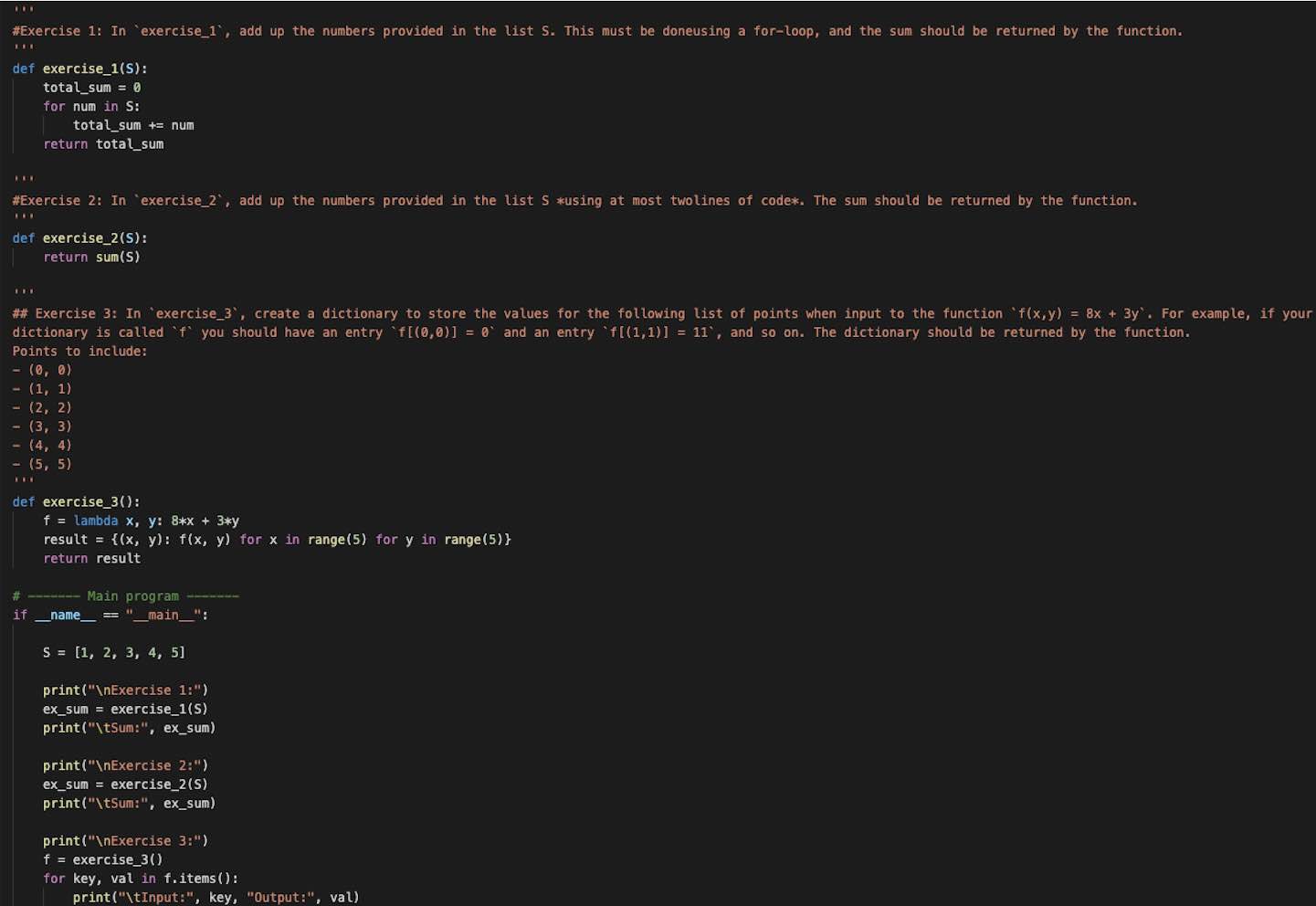
Table of Contents
- Overview
- Getting Started
- D-Wave Tools and Technologies
- Project Summaries
- Older Projects
- Newer Projects
- Contact Information
(BELIEF SPACE)
├── README.md
├── code
│   └── number_partitioning.py
├── data
│   └── training_number_partitioning.json
├── math_equations
│   └── equations.md  ──────
├── results
│   └── sampling_time_analysis.md
└──├── quantum_tsp
│   └── code
│       └── quantum_tsp.py
│   └── data
│       └── cities.json
│   └── math_equations
│       └── tsp_equations.md
│   └── results
│       └── tsp_results.md
├── project_cd24acdf-0a8f-44ae-a150-69ece39acec6
│   ├── code
│   ├── data
│   └── ...
└── project_6dbabf04-9a93-4534-9239-51d9edc7cbe2
    ├── code
    ├── data
    └── ...
# Quantum Computing 101 with D-Wave Systems
This README outlines my journey through a 5-day Quantum Computing 101 lecture series and hands-on training project sessions with D-Wave Systems. In this document, you'll discover my experience working with D-Wave's tools such as D-Wave Inspector and the various types of problems I tackled.
To get started with D-Wave Systems, you will need to:
-
Install D-Wave Ocean SDK: This software stack includes everything you need to build a D-Wave application.
pip install dwave-ocean-sdk
-
Sign Up on D-Wave Leap: D-Wave's cloud service for quantum computing.
- D-Wave Ocean SDK: Primarily used for problem formulation.
- D-Wave IDE: Used for easier problem modeling and solving.
- Qbsolv: For solving QUBO and Ising problems.
- D-Wave Hybrid: For hybrid classical/quantum algorithms.
- Repository: dwavesystems/dwave-inspector
- Language: 100% Python
- License: Apache-2.0 & D-Wave EULA
- Installation:
pip install dwave-inspector
pip install dwave-inspectorapp --extra-index=https://pypi.dwavesys.com/simple
- Description: D-Wave Inspector is a tool for visualizing problems submitted to, and answers received from, a D-Wave structured solver such as an Advantage™ quantum computer.
. ├── project_cd24acdf-0a8f-44ae-a150-69ece39acec6 │ ├── code │ ├── data │ └── ... └── project_6dbabf04-9a93-4534-9239-51d9edc7cbe2 ├── code ├── data └── ...
- Training: Number Partitioning
- Solver: Advantage_system 4.1
- Type: QUBO
- Status: Completed
- Submitted On: 2023-05-18T22:56:57.426472Z
- Solved On: 2023-05-18T22:56:57.597874Z
- Number of Reads: 100
- Submitted By: Zi2q-7cdd45d9...
I utilized the D-Wave Inspector to minor-embed a binary quadratic model onto a Quantum Processing Unit (QPU) for solving a number partitioning problem.
- QPU_SAMPLING_TIME: (10.728 \mathrm{~ms})
- QPU_ANNEAL_TIME_PER_SAMPLE: (20 \mu \mathrm{s})
- QPU_READOUT_TIME_PER_SAMPLE: (67 \mu \mathrm{s})
- QPU_ACCESS_TIME: (26.484 \mathrm{~ms})
- QPU_ACCESS_OVERHEAD_TIME: (580 \mu \mathrm{s})
- QPU_PROGRAMMING_TIME: (15.756 \mathrm{~ms})
- QPU_DELAY_TIME_PER_SAMPLE: (21 \mu \mathrm{s})
- TOTAL_POST_PROCESSING_TIME: (1.895 \mathrm{~ms})
- POST_PROCESSING_OVERHEAD_TIME: (1.895 \mathrm{~ms})
- ID: 23cf353c-5596-4e2e-ab04-dc8372daa7a2
- Type: qubo
- Solver: Advantage_system4.1
- Submitted On: 2023-05-18T23:09:22.949935Z
- Solved On: 2023-05-18T23:09:23.166683Z
- Status: COMPLETED
- Submitted By: Zi2q-7cdd45d9...
- Number of Reads: 100
Plan of Action For Problem
The training project focuses on Number Partitioning. The objective is to partition a set of numbers into two equal subsets such that the sum of the numbers in each subset is as close as possible. This problem is represented as a QUBO optimization problem.
| 1507 | 1522 | 1537 | 1552 | ... | 4403 | energy | num_oc. | |
|---|---|---|---|---|---|---|---|---|
| 0 | 0 | 0 | 0 | 0 | ... | 1 | -9826.5 | 35 |
| 1 | 1 | 1 | 1 | 1 | ... | 0 | -9826.5 | 21 |
| 2 | 1 | 0 | 1 | 1 | ... | 0 | -9816.5 | 24 |
| 3 | 0 | 1 | 0 | 0 | ... | 1 | -9816.5 | 15 |
| 4 | 1 | 1 | 1 | 1 | ... | 0 | -9298.5 | 1 |
| 5 | 1 | 0 | 0 | 0 | ... | 1 | -9276.5 | 1 |
| 6 | 0 | 1 | 1 | 1 | ... | 0 | -9276.5 | 1 |
| 7 | 0 | 0 | 1 | 1 | ... | 0 | -9179.0 | 1 |
| 8 | 1 | 0 | 1 | 1 | ... | 0 | -7332.0 | 1 |
| ... | ... | ... | ... | ... | ... | ... | ... | ... |
- QPU Sampling Time: 10.008 ms
- QPU Anneal Time per Sample: 20 µs
- QPU Readout Time per Sample: 60 µs
- QPU Access Time: 25.764 ms
- QPU Access Overhead Time: 3.494 ms
- QPU Programming Time: 15.756 ms
- QPU Delay Time per Sample: 21 µs
- Post Processing Overhead Time: 3.682 ms
- Total Post Processing Time: 3.682 ms
This training project on Number Partitioning successfully utilizes QUBO optimization to partition a set of numbers into two equal subsets. The energy analysis and sample data provide insights into the optimization results. The timing information highlights the performance characteristics of the solution process.
. ├── project_cd24acdf-0a8f-44ae-a150-69ece39acec6 │ ├── code │ ├── data │ └── ... └── project_6dbabf04-9a93-4534-9239-51d9edc7cbe2 ├── code ├── data └── ...
- Training: Embedding
- Solver: Advantage_system 4.1
- Type: QUBO
- Status: Completed
- Submitted On: 2023-05-18T22:14:41.533053Z
- Solved On: 2023-05-18T22:14:41.702012Z
- Number of Reads: 10
In this project, I focused on learning embedding techniques to better utilize the D-Wave quantum architecture.
- QPU_SAMPLING_TIME: ( t_{\text{sample}} = 11.732 , \mathrm{ms} )
- QPU_ANNEAL_TIME_PER_SAMPLE: ( \tau_{\text{anneal}} = 22 , \mu \mathrm{s} )
- QPU_READOUT_TIME_PER_SAMPLE: ( t_{\text{readout}} = 75 , \mu \mathrm{s} )
- (IN PROGRESS)
ID: f9046ca2-9cc9-40c1-8607-f26e4de62862
SOLVED_ON: 2023-05-18T23:05:11.291053Z
LABEL: Copy Value
STATUS: COMPLETED
SOLVER: Advantage_system 4.1
SUBMITTED_BY: Zi2q-7cdd45d9...
TYPE: qubo
NUM_READS: 100
SUBMITTED_ON: 2023-05-18T23:05:11.109121Z
The training project involved a number partitioning problem. Here is a sample set in JSON format:
[
  {
    "1831": 0,
    "1846": 0,
    "1860": 0,
    "1875": 0,
    "...": "...",
    "3204": 1,
    "energy": -9756.0,
    "num_oc.": 31
  },
  {
    "1831": 1,
    "1846": 1,
    "1860": 1,
    "1875": 1,
    "...": "...",
    "3204": 0,
    "energy": -9756.0,
    "num_oc.": 58
  },
  {
    "1831": 0,
    "1846": 0,
    "1860": 0,
    "1875": 0,
    "...": "...",
    "3204": 1,
    "energy": -9406.0,
    "num_oc.": 1
  },
  {
    "1831": 1,
    "1846": 1,
    "1860": 1,
    "1875": 1,
    "...": "...",
    "3204": 0,
    "energy": -9406.0,
    "num_oc.": 7
  },
  {
    "1831": 0,
    "1846": 0,
    "1860": 0,
    "1875": 0,
    "...": "...",
    "3204": 1,
    "energy": -9067.0,
    "num_oc.": 1
  },
  {
    "1831": 0,
    "1846": 0,
    "1860": 0,
    "1875": 0,
    "...": "...",
    "3204": 1,
    "energy": -9021.0,
    "num_oc.": 1
  },
  {
    "1831": 0,
    "1846": 0,
    "1860": 0,
    "1875": 0,
    "...": "...",
    "3204": 1,
    "energy": -8993.0,
    "num_oc.": 1
  }
]- QPU_SAMPLING_TIME: 9.024 ms
- TOTAL_POST_PROCESSING_TIME: 236 μs
- QPU_ANNEAL_TIME_PER_SAMPLE: 20 μs
- POST_PROCESSING_OVERHEAD_TIME: 236 μs
- QPU_READOUT_TIME_PER_SAMPLE: 50 μs
- QPU_ACCESS_TIME: 24.780 ms
- QPU_ACCESS_OVERHEAD_TIME: 2.061 ms
- QPU_PROGRAMMING_TIME: 15.756 ms
- QPU_DELAY_TIME_PER_SAMPLE: 21 μs
Please note that these performance metrics are indicative of the execution time and overhead involved in solving the number partitioning problem using the Advantage_system 4.1 solver.
For more information on the Advantage_system 4.1 solver, you can refer to the D-Wave website or other relevant resources.
- ID: 10fd40b1-9ef5-4ea0-9e97-2c5a14c2c36d
- The unique identifier for this problem.
- Label: Copy Value
- The label given to this problem.
- Training: Number Partitioning
- The type of training this problem belongs to, which is Number Partitioning in this case.
- Solver: Advantage_system 4.1
- The solver used to solve this problem, which is the Advantage_system 4.1.
- Type: QUBO
- The type of the problem formulation, which is Quadratic Unconstrained Binary Optimization (QUBO) in this case.
- Submitted On: 2023-05-18T23:05:19.742716Z
- The date and time when this problem was submitted.
- Solved On: 2023-05-18T23:05:19.967823Z
- The date and time when this problem was solved.
- Status: COMPLETED
- The status of this problem, which is COMPLETED.
- Submitted By: Zi2q-7cdd45d9...
- The identifier of the user who submitted this problem.
- Num Reads: 100
- The number of reads performed on the solver.
- QPU Sampling Time: 11.640 ms
- The total time taken by the Quantum Processing Unit (QPU) to perform the sampling operation, which is 11.640 milliseconds.
- QPU Anneal Time per Sample: 20 μs
- The time taken by the QPU for each sample during the annealing process, which is 20 microseconds.
- QPU Readout Time per Sample: 76 μs
- The time taken by the QPU for each sample during the readout process, which is 76 microseconds.
- QPU Access Time: 27.397 ms
- The total time taken to access the QPU, including annealing time, readout time, and other overheads, which is 27.397 milliseconds.
- QPU Access Overhead Time: 1.938 ms
- The overhead time incurred while accessing the QPU, which is 1.938 milliseconds.
- QPU Programming Time: 15.757 ms
- The time taken to program the QPU with the problem, which is 15.757 milliseconds.
- QPU Delay Time per Sample: 21 μs
- The delay time between each sample during the QPU operation, which is 21 microseconds.
- Post Processing Overhead Time: 427 μs
- The overhead time incurred during post-processing, which is 427 microseconds.
- Total Post Processing Time: 427 μs
- The total time taken for post-processing, which is 427 microseconds.
- ID: 4838543d-7640-4f98-ba84-45d171c10911
- Solver: Advantage_system4.1
- Type: qubo
- Status: Completed
- Submitted By: Zi2q-7cdd45d9...
- Number of Reads: 100
The results were exported in a JSON format, showcasing various energy levels and number occurrences:
[ \begin{array}{lrrrrlrrr} & 2465 & 2480 & 2495 & 2510 & \ldots & 4048 & \text{energy} & \text{num_oc} \ 0 & 0 & 0 & 0 & 0 & \ldots & 1 & -9713.0 & 21 \ 1 & 1 & 1 & 1 & 1 & \ldots & 0 & -9713.0 & 41 \ ... 15 & 1 & 1 & 1 & 1 & \ldots & 0 & -8735.0 & 1 \ \end{array} ]
- QPU Sampling Time: 12.560 ms
- Post-Processing Overhead Time: 2.014 ms
- QPU Anneal Time per Sample: 20 µs
- Total Post-Processing Time: 2.014 ms
- QPU Readout Time per Sample: 85 µs
- QPU Access Time: 28.316 ms
- QPU Access Overhead Time: 7.735 ms
- QPU Programming Time: 15.756 ms
- QPU Delay Time per Sample: 21 µs
This project aims to solve the Number Partitioning problem by using D-Wave's quantum annealing technology.
Mathematical Background: The Number Partitioning problem can be represented as a QUBO (Quadratic Unconstrained Binary Optimization) problem with a Hamiltonian ( H = \sum_{i,j} a_{ij} x_i x_j ), where ( x_i ) are binary variables and ( a_{ij} ) are elements of a matrix that represents the problem constraints.
- Python3
- Ocean SDK
- D-Wave Leap Quantum Cloud Service
- Problem Formulation: Transform the Number Partitioning problem into a QUBO problem.
- Quantum Annealing: Utilize D-Wave's quantum annealer to find the optimal solution.
- Data Analysis: Analyze the output for different problem instances.
The results were represented in terms of binary variables and energy states:
| Index | 702 | 732 | 747 | 762 | 777 | ... | 5238 | Energy |
|---|---|---|---|---|---|---|---|---|
| 0 | 0 | 0 | 0 | 1 | 0 | ... | 1 | -6889.0 |
| 1 | 1 | 1 | 1 | 0 | 1 | ... | 0 | -6889.0 |
| ... | ... | ... | ... | ... | ... | ... | ... | ... |
Mathematical Insight: The energy values indicate the quality of the solutions. Lower energy values represent better solutions according to the Hamiltonian ( H ).
- QPU Sampling Time: (11.688 , \text{ms})
- Post-Processing Overhead Time: (3.737 , \text{ms})
- QPU Anneal Time Per Sample: (20 , \mu \text{s})
- Total Post-Processing Time: ( ... )
Here is an illustrative Python3 snippet for formulating the QUBO matrix:
from dimod import BinaryQuadraticModel

# Create an empty Binary Quadratic Model
bqm = BinaryQuadraticModel('BINARY')

# Define QUBO interactions (Example values)
qubo_interactions = {(0, 0): -1, (1, 1): -1, (0, 1): 2}

# Add interactions to BQM
bqm.add_interactions_from(qubo_interactions)
The above code sets up the QUBO matrix to represent the problem on the D-Wave quantum annealer.
Title:
Training - Number Partitioning
ID:
79d129a2-12c3-4577-b14d-a5be2aa595a2
Solver Used:
Advantage_system4.1
Type:
QUBO (Quadratic Unconstrained Binary Optimization)
Status:
COMPLETED
Submitted On:
2023-05-18T23:13:34.598117Z
Solved On:
2023-05-18T23:13:34.772877Z
Submitted By:
Zi2q-7cdd45d9...
Number of Reads:
100
- QPU Sampling Time:
( 14.184 , \text{ms} ) - Post-Processing Overhead Time:
( 815 , \mu \text{s} )
- QPU Anneal Time Per Sample:
( 20 , \mu \text{s} ) - Total Post-Processing Time:
( 815 , \mu \text{s} ) - QPU Readout Time Per Sample:
( 101 , \mu \text{s} )
- QPU Access Time:
( 29.940 , \text{ms} ) - QPU Access Overhead Time:
( 2.744 , \text{ms} ) - QPU Programming Time:
( 15.756 , \text{ms} ) - QPU Delay Time Per Sample:
( 21 , \mu \text{s} )
- Solver: Advantage_system4.1
- Type: QUBO
- ID: aOc53d79-eab6-4661-8449-69d7c667fadb
- Submitted On: 2023-05-18T23:24:01.849039Z
- Solved On: 2023-05-18T23:24:02.052210Z
- Status: Completed
- Submitted By: Zi2q-7cdd45d9...
- Number of Reads: 100
[ \begin{align*} \text{QPU Sampling Time} &: 10.704 , \text{ms} \ \text{QPU Anneal Time per Sample} &: 20 , \mu \text{s} \ \text{QPU Readout Time per Sample} &: 67 , \mu \text{s} \ \text{QPU Access Time} &: 26.462 , \text{ms} \ \text{QPU Access Overhead Time} &: 516 , \mu \text{s} \ \text{QPU Programming Time} &: 15.758 , \text{ms} \ \text{QPU Delay Time per Sample} &: 21 , \mu \text{s} \ \text{Post-Processing Overhead Time} &: 1.927 , \text{ms} \ \text{Total Post-Processing Time} &: 1.927 , \text{ms} \ \end{align*} ]
Here are some of the optimized solutions:
[ \begin{array}{cccc} 1899 & 1914 & 1929 & \ldots \ 0 & 1 & 0 & \ldots \ \vdots & \vdots & \vdots & \ddots \ \end{array} ]
Energy Level: -6889.0 to -6355.94833
- Project ID: d54e319b-20ba-4fdd-8341-aa8430e83fbb
- Solver: Advantage_system4.1
- Type: QUBO (Quadratic Unconstrained Binary Optimization)
- Submitted On: 2023-05-18
- Solved On: 2023-05-18
- Status: COMPLETED
- Submitted By: Zi2q-7cdd45d9...
- Number of Reads: 100
- QPU Sampling Time: N/A
- Post-Processing Overhead Time: 9.264 ms
- Total Post-Processing Time: 711μs
- QPU Readout Time Per Sample: 52μs
- QPU Access Time: 25.022 ms
- QPU Access Overhead Time: 827μs
- QPU Programming Time: 15.758 ms
- QPU Delay Time Per Sample: 21μs
The output energies ranged from -6889.0 to -6313.0, with varying numbers of occurrences for each unique solution.
| Energy | Number of Occurrences |
|---|---|
| -6889.0 | 2 |
| -6888.0 | 16 |
| -6880.0 | 15 |
| ... | ... |
| -6313.0 | 1 |
The Python code to retrieve and process the quantum results was as follows.
# Python code to process D-Wave output
from dwave.system import DWaveSampler, EmbeddingComposite

# Initialize sampler and composite
sampler = DWaveSampler(solver={'qpu': True})
composite = EmbeddingComposite(sampler)

# Define QUBO problem (example)
Q = {(0, 0): -1, (1, 1): -1, (0, 1): 2}

# Sample
sampleset = composite.sample_qubo(Q, num_reads=100)

# Process results
for sample, energy, occurrences in sampleset.data(['sample', 'energy', 'num_occurrences']):
print(sample, "Energy:", energy, "Occurrences:", occurrences)The energy function ( E ) in a QUBO problem is given by
[ E = \sum_{i} q_{i} x_{i} + \sum_{i < j} q_{ij} x_{i} x_{j} ]
Here, ( q_{i} ) and ( q_{ij} ) are coefficients of the QUBO matrix, and ( x_{i} ) are binary variables (0 or 1).
# D-Wave Systems Quantum Computing: Session 2


## Project Details

### Problem Statement
The optimization problem remains in the QUBO framework, which is ideal for solving problems like the Traveling Salesman Problem, Maximum Cut, etc.

### Solution Methodology
The problem was solved using the Quantum Annealing algorithm, optimized using the QUBO method.


## Solver Metrics

### Basic Metrics
- **Solver**: Advantage_system4.1
- **Type**: qubo
- **Status**: COMPLETED
- **Submitted By**: Zi2q-7cdd45d9...
- **ID**: cb05cbd3-e180-4919-958a-98b2a95bb94d

### Timing Metrics
- **QPU Sampling Time**: \(8.176 \, \text{ms}\)
- **QPU Anneal Time Per Sample**: \(20 \, \mu \text{s}\)
- **QPU Readout Time Per Sample**: \(41 \, \mu \text{s}\)
- **QPU Access Time**: \(23.937 \, \text{ms}\)
- **QPU Access Overhead Time**: \(1.503 \, \text{ms}\)
- **QPU Programming Time**: \(15.761 \, \text{ms}\)
- **QPU Delay Time Per Sample**: \(21 \, \mu \text{s}\)
- **Total Post-Processing Time**: \(802 \, \mu \text{s}\)
- **Post-Processing Overhead Time**: \(802 \, \mu \text{s}\)


## Results and Analysis

The output results show different configurations with respective energies and occurrences. The lowest energy configuration is our area of interest.
| 1144 | 1234 | 3846 | 3905 | energy | num_oc. |
|---|---|---|---|---|---|
| 0 | 1 | 1 | 0 | -1.0 | 53 |
| 0 | 1 | 1 | 1 | -1.0 | 47 |
## Mathematical Context

The energy function \(E\) can be expressed as:

\[
E(x) = \sum_{i=1}^{4} \sum_{j=1}^{4} Q_{ij} x_i x_j
\]

Here, \(Q_{ij}\) represents the coefficients in the QUBO problem, and \(x_i\) are the binary variables. Minimizing \(E(x)\) provides us with the optimal solution.


## Python3 Code

Here's a Python3 example using D-Wave's SDK:

```python
from dwave.system import DWaveSampler, EmbeddingComposite

# Define the QUBO dictionary
Q = {(1144, 1144): 1, (1234, 1234): -2, (3846, 3846): 3, (3905, 3905): -4}

# Use the D-Wave sampler
sampler = EmbeddingComposite(DWaveSampler())
response = sampler.sample_qubo(Q, num_reads=100)

# Output results
for sample, energy, num_oc in response.data(['sample', 'energy', 'num_occurrences']):
    print(sample, "Energy: ", energy, "Occurrences: ", num_oc)
The objective of this project was to explore the quantum annealing capabilities for solving number partitioning problems. Number partitioning is a computationally complex problem and provides an excellent use-case for quantum computing.
We utilized D-Wave's Quantum Annealing Solver to solve the given problem. The optimization process was carried out using the Quadratic Unconstrained Binary Optimization (QUBO) framework.
- Solver: Advantage_system4.1
- Type: qubo
- Status: COMPLETED
- Submitted By: Zi2q-7cdd45d9...
- ID: 98fd1adb-7c4e-48e2-9172-8513b098d505
- QPU Sampling Time: 9.040 ms
- QPU Anneal Time Per Sample: 20 µs
- QPU Readout Time Per Sample: 50 µs
- QPU Access Time: 24.801 ms
- QPU Access Overhead Time: 2.498 ms
- QPU Programming Time: 15.761 ms
- QPU Delay Time Per Sample: 21 µs
- Total Post-Processing Time: 587 µs
- Post-Processing Overhead Time: 587 µs
The QUBO problem was solved using 100 reads, and the output included several configurations with different energy levels. The lowest energy configuration provides the most optimal solution.
energy  | num_oc. | 2473 | 2488 | 2503 | ... | 5428
--------|---------|------|------|------|-----|------
-6889.0 |    1    |  0   |  0   |  0   | ... |  1
-6889.0 |    1    |  0   |  1   |  0   | ... |  0
-6888.0 |    4    |  1   |  1   |  0   | ... |  1
...     |   ...   | ...  | ...  | ...  | ... | ...
The energy function (E) in QUBO is usually represented as:
Here is a sample Python3 code snippet to perform a quantum annealing task using D-Wave's Python SDK:
from dwave.system import DWaveSampler, EmbeddingComposite

# Define QUBO dictionary
Q = {(0, 0): -1, (0, 1): 2, (1, 1): -1}
sampler = EmbeddingComposite(DWaveSampler())
response = sampler.sample_qubo(Q, num_reads=100)

# Extract results
for sample, energy, num_oc in response.data(['sample', 'energy', 'num_occurrences']):
print(sample, "Energy: ", energy, "Occurrences: ", num_oc)We utilized D-Wave's Quantum Annealing Solver to solve the given problem. The optimization process was carried out using the Quadratic Unconstrained Binary Optimization (QUBO) framework.
- Solver: Advantage_system4.1
- Type: qubo
- Status: COMPLETED
- Submitted By: Zi2q-7cdd45d9...
- ID: 98fd1adb-7c4e-48e2-9172-8513b098d505
- QPU Sampling Time: 9.040 ms
- QPU Anneal Time Per Sample: 20 µs
- QPU Readout Time Per Sample: 50 µs
- QPU Access Time: 24.801 ms
- QPU Access Overhead Time: 2.498 ms
- QPU Programming Time: 15.761 ms
- QPU Delay Time Per Sample: 21 µs
- Total Post-Processing Time: 587 µs
- Post-Processing Overhead Time: 587 µs
The QUBO problem was solved using 100 reads, and the output included several configurations with different energy levels. The lowest energy configuration provides the most optimal solution.
energy  | num_oc. | 2473 | 2488 | 2503 | ... | 5428
--------|---------|------|------|------|-----|------
-6889.0 |    1    |  0   |  0   |  0   | ... |  1
-6889.0 |    1    |  0   |  1   |  0   | ... |  0
-6888.0 |    4    |  1   |  1   |  0   | ... |  1
...     |   ...   | ...  | ...  | ...  | ... | ...
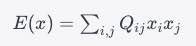
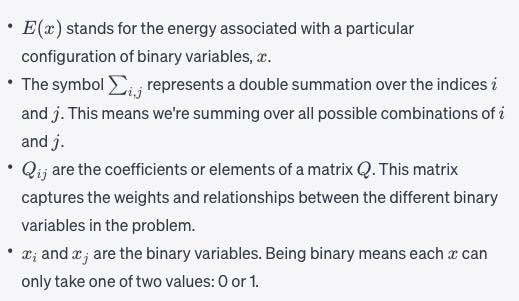
The energy function (E) in QUBO is usually represented as:
[ E(x) = \sum_{i,j} Q_{ij} x_i x_j ]
where (Q_{ij}) are the elements of a QUBO matrix and (x_i, x_j) are the binary variables. The objective is to find (x) that minimizes (E(x)).
Here is a sample Python3 code snippet to perform a quantum annealing task using D-Wave's Python SDK:
from dwave.system import DWaveSampler, EmbeddingComposite

# Define QUBO dictionary
Q = {(0, 0): -1, (0, 1): 2, (1, 1): -1}
sampler = EmbeddingComposite(DWaveSampler())
response = sampler.sample_qubo(Q, num_reads=100)

# Extract results
for sample, energy, num_oc in response.data(['sample', 'energy', 'num_occurrences']):
    print(sample, "Energy: ", energy, "Occurrences: ", num_oc)
# D-Wave Systems Quantum Computing: Session 2
## Table of Contents
1. [Overview](#overview)
2. [Project Details](#project-details)
3. [Solver Metrics](#solver-metrics)
4. [Results and Analysis](#results-and-analysis)
5. [Mathematical Context](#mathematical-context)
6. [Python3 Code](#python3-code)
## Project Details
### Problem Statement
The optimization problem remains in the QUBO framework, which is ideal for solving problems like the Traveling Salesman Problem, Maximum Cut, etc.
### Solution Methodology
The problem was solved using the Quantum Annealing algorithm, optimized using the QUBO method. Larger graphs are formulated as QUBOs for hybrid classical quantum qbsolv - 0/1 valued variables
Minimizing the objective function:

$$
O(Q, x)=\Sigma Q_{i i} x_i+\Sigma q_{i j} x_i x_j
$$
## Solver Metrics
### Basic Metrics
- **Solver**: Advantage_system4.1
- **Type**: qubo
- **Status**: COMPLETED
- **Submitted By**: Zi2q-7cdd45d9...
- **ID**: cb05cbd3-e180-4919-958a-98b2a95bb94d
### Timing Metrics
- **QPU Sampling Time**: \(8.176 \, \text{ms}\)
- **QPU Anneal Time Per Sample**: \(20 \, \mu \text{s}\)
- **QPU Readout Time Per Sample**: \(41 \, \mu \text{s}\)
- **QPU Access Time**: \(23.937 \, \text{ms}\)
- **QPU Access Overhead Time**: \(1.503 \, \text{ms}\)
- **QPU Programming Time**: \(15.761 \, \text{ms}\)
- **QPU Delay Time Per Sample**: \(21 \, \mu \text{s}\)
- **Total Post-Processing Time**: \(802 \, \mu \text{s}\)
- **Post-Processing Overhead Time**: \(802 \, \mu \text{s}\)
## Results and Analysis
The output results show different configurations with respective energies and occurrences. The lowest energy configuration is our area of interest.
| 1144 | 1234 | 3846 | 3905 | energy | num_oc. |
|---|---|---|---|---|---|
| 0 | 1 | 1 | 0 | -1.0 | 53 |
| 0 | 1 | 1 | 1 | -1.0 | 47 |
## Python3 Code

Python3 example using D-Wave's SDK:

```python
from dwave.system import DWaveSampler, EmbeddingComposite

# Define the QUBO dictionary
Q = {(1144, 1144): 1, (1234, 1234): -2, (3846, 3846): 3, (3905, 3905): -4}

# Use the D-Wave sampler
sampler = EmbeddingComposite(DWaveSampler())
response = sampler.sample_qubo(Q, num_reads=100)

# Output results
for sample, energy, num_oc in response.data(['sample', 'energy', 'num_occurrences']):
    print(sample, "Energy: ", energy, "Occurrences: ", num_oc)
## Project Summary
**Problem Statement:** Quantum Optimization for Real-world Problems
**Solution Methodology:** Quantum Annealing
**Solver Used:** D-Wave Advantage_system4.1
**Status:** Completed


## Technologies
- Python 3
- D-Wave Ocean SDK
- NumPy
- Mathematical Formulation (QUBO)


## Solver Metrics

### Basic Metrics
- **Solver**: Advantage_system4.1
- **Type**: qubo
- **Status**: COMPLETED
- **ID**: d1d2971f-70f0-4db4-aec4-7cb25734aedb
- **Submitted By**: Zi2q-7cdd45d9...
- **Submitted On**: 2023-05-19T02:46:11.148532Z
- **Num Reads**: 100

### Timing Metrics
- **QPU Sampling Time**: \(9.346 \, \text{ms}\)
- **QPU Anneal Time Per Sample**: \(20 \, \mu \text{s}\)
- **QPU Readout Time Per Sample**: \(53 \, \mu \text{s}\)
- **QPU Access Time**: \(25.107 \, \text{ms}\)
- **QPU Access Overhead Time**: \(1.258 \, \text{ms}\)
- **QPU Programming Time**: \(15.761 \, \text{ms}\)
- **QPU Delay Time Per Sample**: \(21 \, \mu \text{s}\)
- **Total Post-Processing Time**: \(3.709 \, \text{ms}\)
- **Post-Processing Overhead Time**: \(3.709 \, \text{ms}\)


## Results

The output was an optimal solution for our problem with the following attributes:

\[
\begin{aligned}
& 173243134463 \quad \text {energy num_oc.} \\
& 0 \quad 1 \quad 1 \quad 0 \quad -1.0 \quad 100 \\
\end{aligned}
\]


## Mathematical Context

The energy function \(E\) can be modeled as:

\[
E(x) = \sum_{i=1}^{n} \sum_{j=1}^{n} Q_{ij} x_i x_j
\]

where \(Q_{ij}\) are the coefficients in the QUBO problem, and \(x_i\) are the binary variables.


##  Code


```python
# Sample Python code using D-Wave SDK
from dwave.system import DWaveSampler, EmbeddingComposite
Q = {(0, 0): 1, (1, 1): -1, (2, 2): 1}
sampler = EmbeddingComposite(DWaveSampler())
response = sampler.sample_qubo(Q, num_reads=100)
## Project ID: a4253abc-9a1b-4b8f-b5e3-4fb85b11cfdf
### Meta Information
- **Solver**: Advantage_system4.1
- **Type**: qubo
- **Submitted On**: 2023-05-18T20:10:44.740770Z
- **Solved On**: 2023-05-18T20:10:45.314233Z
- **Status**: COMPLETED
- **Submitted By**: Zi2q-7cdd45d9...
- **Number of Reads**: 10
### Project Overview
### Results
```latex
\begin{aligned}
& 997 1012 1042 4309 4340 4385 4400 \text{ energy num_oc. } \\
& 0 0 0 1 1 0 1 -3.0 1 \\
& 1 0 1 0 0 1 1 0 -3.0 5 \\
& 2 0 1 0 0 1 0 1 -3.0 2 \\
& 3 0 0 0 1 1 1 0 -3.0 2 \\
& \text{['BINARY', 4 rows, 10 samples, 7 variables]}
\end{aligned}- QPU Sampling Time: 891 µs
- Total Post-Processing Time: 141 µs
- QPU Anneal Time per Sample: 141 µs
- Post-Processing Overhead Time: 141 µs
- QPU Readout Time per Sample: 49 µs
- QPU Access Time: 16.649 ms
- QPU Access Overhead Time: 741 µs
- QPU Programming Time: 15.757 ms
- QPU Delay Time per Sample: 21 µs
---
## Projects
### Graph Mapping with D-Wave Systems
](https://ide.dwavesys.io/#https://github.com/dwave-training/graph-mapping)
**Overview**:
This project leverages D-Wave Systems to solve graph mapping problems. Specifically, it aims to solve the antenna selection problem using quantum annealing.
#### Exercise Highlights
- **Exercise 1**: Initialization
- Token authentication for D-Wave's Leap IDE.
- Introduction to `dwave-networkx`.
- **Exercise 2**: Simulated Annealing
- Implementing the simulated annealing algorithm.
- **Exercise 3**: Problem Modification
- Modified the original problem to solve for minimum vertex cover.
#### Core Technologies
- NetworkX
- D-Wave NetworkX
- D-Wave System's QPU
- Matplotlib for visualization
#### Code Snippets
```python
# Importing essential packages
import networkx as nx
from dwave.system import DWaveSampler, EmbeddingComposite
# Creating the graph structure
G = nx.Graph()
G.add_edges_from([(1, 2), (1, 3), (2, 3), (3, 4), (3, 5), (4, 5), (4, 6), (5, 6), (6, 7)])
# Defining sampler
sampler = EmbeddingComposite(DWaveSampler())
- Python
- D-Wave Systems
- NetworkX
- Matplotlib
- Leap IDE
Feel free to connect with me:
- 📧 Email: davidmerwin1992@gmail.com
- 💼 LinkedIn:
- 🌐 Portfolio: D-Wave Profile
Thank you for visiting my portfolio! 😊
Feel free to reach out if you have any questions or would like to collaborate!