bayes.js is small toy JavaScript MCMC framework that can be used fit Bayesian models in the browser. I call it "toy" because I would use it for fun, but not in production...
The two major files are:
- mcmc.js - Implements a MCMC framework which can be used to fit Bayesian model with both discrete and continuous parameters. Currently the only algorithm that is implemented is a version of the adaptive Metropolis within Gibbs (AMWG) algorithm presented by Roberts and Rosenthal (2009) . Loading this file in the browser creates the global object
mcmc. - distributions.js - A collection of log density functions that can be used to construct Bayesian models. Follows the naming scheme
ld.*(for example,ld.normandld.pois) and uses the same parameters as thed*density functions in R. Loading this file in the browser creates the global objectld.
In addition to this the whole thing is wrapped in an Rstudio project as I've use R and JAGS to write some tests.
Given that mcmc.js and distributions.js have been imported, here is how to define a model assuming a Normal distribution, and fit it to some data and produce a sample of 5000 draws from the posterior:
// The heights of the last ten American presidents in cm, from Kennedy to Obama
var data = [183, 192, 182, 183, 177, 185, 188, 188, 182, 185];

var params = {
  mu: {type: "real"},
  sigma: {type: "real", lower: 0} };

var log_post = function(state, data) {
  var log_post = 0;
  // Priors
  log_post += ld.norm(state.mu, 0, 100);
  log_post += ld.unif(state.sigma, 0, 100);
  // Likelihood
  for(var i = 0; i < data.length; i++) {
    log_post += ld.norm(data[i], state.mu, state.sigma);
  }
  return log_post;
};

// Initializing the sampler
var sampler =  new mcmc.AmwgSampler(params, log_post, data);
// Burning some samples to the MCMC gods and sampling 5000 draws.
sampler.burn(1000)
var samples = sampler.sample(5000)
You can find an interactive version of this script here
And here is a plot of the resulting sample made in JavaScript using the plotly.js library:

In mcmc.js the currently sole sampler is AmwgSampler: An adaptive, general purpose MCMC sampler that can be used to fit a wide range of models in theory. In practice AmwgSampler can work well as long as there are not too many parameters. Here it's hard to specify what is "too many" but generally <10 parameters should be fine but >100 might be too many, but it depends. As AmwgSampler is a Gibbs sampler it also becomes crippled when the parameters are correlated.
Here is how to create an instance of AmwgSampler and produce a number of samples from a model defined by params and log_post:
var sampler = new mcmc.AmwgSampler(params, log_post, data);
var samples = sampler.sample(1000)
The four arguments to AmwgSampler are:
params: This is an object that specifies the parameters in the model.
log_post: A function that defines the model, were the first argument is the state of the parameters and the second is an optional data argument, and which should return a number proportional to the log posterior.
data (optional): An optional argument, whatever you pass in here will just be passed on to the log_post function.
options (optional): An object defining options to the sampler.
Let's go through them in order!
This is an object that describes the parameters in the model by giving the parameter names as keys and the parameter properties as objects. The following would define the parameters of a Normal distribution:
params = {
  mu:    {type: "real", dim: [1], lower: -Infinity, upper: Infinity, init: 0.5 },
  sigma: {type: "real", dim: [1], lower:  0,        upper: Infinity, init: 0.5 }};
There are five parameter properties:
type- a string that defines the type of parameter. Can be"real","int"or"binary". Note that this has nothing to do with JavaScript types, it's just to inform the sampler how to handle the parameter.dim- an array giving the dimensions of the parameter. For exampledim: [1]would define a scalar (a single number),dim: [3]a vector of length 3, anddim: [2,2]a 2 by 2 matrix.lower- A number giving the lower support of the parameter.upper- A number giving the upper support of the parameter.init- A number or an array giving the initial value of the parameter when starting the sampler.
Not all parameter properties need to be filled in and when left out will be replaced by defaults, for example, the following will result in the same parameter definition as above:
params = {mu: {}, sigma: {lower:0}}If no type is given it defaults to "real" and otherwise the default parameter properties depend on the type. The following...
params = {
  a: {},
  b: {type: "real"},
  c: {type: "int"},
  d: {type: "binary"}};
... would define the same parameters as below:
params = {
  a: {type: "real",   dim: [1], lower: -Infinity, upper: Infinity, init: 0.5},
  b: {type: "real",   dim: [1], lower: -Infinity, upper: Infinity, init: 0.5},
  c: {type: "int",    dim: [1], lower: -Infinity, upper: Infinity, init: 1},
d: {type: "binary", dim: [1], lower: 0, upper: 1, init: 1}};This is a function that defines your model. It should take two arguments, the state of the parameters and the data (but you can leave out the data if your model doesn't use any). The function should return a number proportional to the log posterior density of that state-parameter combination. The data will have whatever format you pass in when you instantiate the sampler, but the format of the state will depend on the parameter definition.
The state is an object which has one element for each parameter with the parameter names as keys and the parameter states as values. The states of one-dimensional (dim: [1]) parameters will be numbers while the states of multi-dimensional parameters will be arrays of numbers.
For example, the following parameter definition...
params = {
  intercept: {type: "real"},
  beta:      {type: "real",   dim: [3]},
  bin_mat:   {type: "binary", dim: [2, 3]} };
... would result in the following state (except for that the specific values could be different, of course):
state = {
  intercept: 0.6,
  beta:      [0.2, -0.5, 10.5],
  bin_mat:   [[1, 1, 0], [0, 0, 1], [1, 1, 1]];
In order to calculate the log posterior it's useful to have access to functions that return the log density of a bunch of probability distributions. This can be found in the distributions.js file which when imported creates a global object ld that contains a number of log density functions, for example ld.norm, ld.beta, and ld.pois.
The design pattern for crafting a log posterior function goes something like this (here exemplified by a standard beta Bernoulli model) :
var log_post = function(state, data) {
// Start by defining a variable to hold the log posterior initialized to 0
var log_post = 0;
// Add the log densities of the priors to log_post.
// If Priors are not specified it is the same as assuming flat uniform priors.
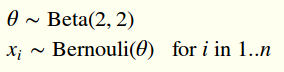
log_post += ld.beta(state.theta, 2, 2);
// Loop through the data and add each resulting log density to log_post.
var n = data.x.length;
for(var i = 0; i < n; i++) {
log_post += ld.bern(data.x[i], state.theta)
}
return log_post;
}The function above corresponds to the following model:
In this section I've used the variable names state and data but you are free to use whatever names you want, what matters is that the first argument is the state and the second argument is the data.
This is easy, whatever you pass in as the data argument when instantiating an AmwgSampler will be passed on to the log posterior function (log_post). So it's up to you what kind of data structure you want to work with in log_post.
There are a bunch of options that can be given to AmwgSampler as an options object, for example:
thin- an integer specifying the number of steps between each saved sample. Defaults to 1.0.monitor- an array of strings specifying what parameters to monitor and return samples from. Defaults tonullwhich means that all parameters will be monitored.
It is also possible to control how the sampler adapts it's proposal, where the most important options are:
prop_log_scale- The initial log(SD) of the one-dimensional proposal (using the same initial log(SD) for each parameter). Defaults to 0.0 which implies a SD of exp(0) == 1.0.target_accept_rate- The acceptance rate of the proposals the sampler tries to achieve. Defaults to 0.44.batch_size- The number of steps between each update of theprop_log_scale. Defaults to 50.max_adaptation- The maximum amountprop_log_scaleis changed each batch update. Defaults to 0.33.
If you want to know more about what these settings do I urge you to read the rather accessible paper by Roberts and Rosenthal (2009) . These options can also be given to specific parameters by supplying a params value overriding options for one or more parameters. For example, var options = {max_adaptation: 0.5, params: { mu: {max_adaptation: 0.1} } } would use max_adaptation: 0.5 for all parameters except for mu which would get max_adaptation: 0.1.
So, using the beta-Bernoulli log_dens function defined above we could define and fit this model like this:
var data = {x: [1, 0, 1, 1, 0, 1, 1, 1]}
var params = {theta: {type: "real", lower: 0, upper: 1}}
var options = {thin: 2} // Not really necessary to thin here, just showin' how...
var sampler = new mcmc.AmwgSampler(params, log_post, data, options);
var samples = sampler.sample(1000);
You can find an interactive version of this script here.
Here are some interactive examples implemented as Codepens that should run in the browser.
- A Normal distribution
- A Bernouli distribution with a Beta prior.
- A Bernouli model with a spike-n-slab prior
- An analysis of capture-recapture data
- Correlation analysis / bivariate Normal model
- Simple linear regression
- Multivariate logistic regression
- A Poisson rate change point analysis
- the "Pump" example from the BUGS project
- An hierarchical model with varying slope and intercept from Gelman and Hill (2006) (This is stretching the limits of what the simple
AmwgSamplercan do...)
These demos rely on the plotly.js library and I haven't tested them extensively on different platforms/browsers. You should be able to change the data and model definition on the fly (but if you change some stuff, like adding multidimensional variables, the plotting might stop working).
The file distributions.js implements log densities for most of the common probability distributions. The log density functions use the naming scheme of R when possible but are not vectorized in any way. Some of the implemented distributions are:
- Bernoulli distribution:
ld.bern(x, prob) - Binomial distribution:
ld.binom(x, size, prob) - Poisson distribution:
ld.pois(x, lambda) - Normal distribution:
ld.norm(x, mean, sd) - Laplace distribution:
ld.laplace(x, location, scale) - Gamma distribution:
ld.gamma(x, shape, rate) - Bivariate normal distribution parameterized by correlation:
bivarnorm(x, mean, sd, corr)
For the full list of distributions just check the source of distributions.js.
- When is a JavaScript MCMC sampler useful?
- Well, for starters, it's not particularly useful if you want to do serious Bayesian data analysis. Then you should use a serious tool like JAGS or STAN. It could, however, be useful if you would want to put a demo of a Bayesian model online, but don't want to / can't run the computations on a server. It could also be useful as a part of a JavaScript application making use of Bayesian computation at some point.
- How good is the sampler that bayes.js uses?
- bayes.js implements the adaptive Metropolis within Gibbs described by Roberts and Rosenthal (2009) which is a good algorithm in that (1) it's adaptive and works out-of-the-box without you having to set a lot of tuning parameters, (2) it can handle both continuous and discrete parameters, (3) it is easy to implement. The downside with the sampler is that (1) it only works well with a small number of parameters, (2) it's a Gibbs sampler so it's going to struggle with correlated parameters.
- What is "a small number of parameters"?
- Depends heavily on context but <10 is probably "small" here. But depending on the model you're trying to run you might get away with 100+ parameters.
- How fast is it?
- Also super context dependent. On simple models it's pretty fast, for example, fitting a standard Normal model on 1000 datapoints producing a sample of 20,000 draws takes ~0.5 s. on my computer. Also, when I've been playing around with different browsers I've seen order-of-magnitude changes in performance when changing seemingly arbitrary things. For example, inlining the definition of the Normal density in the function calculating the log posterior rather than using
ld.normdefined in distributions.js resulted in 10x slower sampling on Firefox 37.
- Also super context dependent. On simple models it's pretty fast, for example, fitting a standard Normal model on 1000 datapoints producing a sample of 20,000 draws takes ~0.5 s. on my computer. Also, when I've been playing around with different browsers I've seen order-of-magnitude changes in performance when changing seemingly arbitrary things. For example, inlining the definition of the Normal density in the function calculating the log posterior rather than using
- Are there any alternatives if I want to do Bayes in the browser?
- There's a probibalistic programming language called webppl that's implemented in JavaScript and that looks great, but I don't have any experience using it.
The sampler as defined in mcmc.js is somewhat over-engineered as it includes a little "framework" of classes for implementing new sampling algorithms. The two main type of classes are Steppers and Samplers. A Stepper is a class responsible for moving one or more parameters around in parameter space. A Sampler is a more "user facing" class that handles the setup of a collection of Steppers that together takes a full step in the model's parameter space. Here AmwgSampler is so far the only implemented Sampler. For more details just check the source of mcmcm.js which is not completely absent of comments.
bayes.js is wrapped inside an Rstudio project and that's because I've used R to compare and test the performance of mcmc.js and distributions.js. I've also implemented a number of unit tests, however, many of those tests check that the samples of bayes.js have the right distribution but because the samples are random draws these tests actually fail from time to time. Having tests that fail even if noting is wrong is not ideal, but it's better than no tests at all I figured...
Roberts, G. O., & Rosenthal, J. S. (2009). Examples of adaptive MCMC. Journal of Computational and Graphical Statistics, 18(2), 349-367. pdf